QChem Tutorial
Optimization and frequency
Let’s take a guess geometry for the water molecule and put it in h2o.xyz:
3

H   0.76144678642012      0.42041157793785     -0.21139612912752
O   0.00092389677508     -0.10975434825824      0.05112764711589
H   -0.76825069319520      0.42203277032039     -0.18105150798837
In this tutorial we are going to use the single opt-freq input, that consists in an initial hessian calculation, followed by an optimization and finally by a frequency calculation. We create the input file using bulma:
python bulma.py h2o.xyz --qchem-opt-freq --BS def2-QZVP
In this tutorial, we are not going to use the default basis set (def2-TZVP), so we include the --BS flag. As a remainder, bulma adapts only some tags, so some methods and basis sets require the correct, verbatim string in input, as in this tutorial.
We recommend to include the -save option when running QChem, otherwise the scratch folder will not be saved and the HESS file will be lost:
qchem -save -np <# proc.> <input> <output>
NB: only the DFT methods print the HESS file. The expansion of bulma to QChem post-HF methods is still WIP.
When the job is terminated, we extract the hessian, that should be printed by QChem in the HESS file located in the folder <outdir>/qchem_scratch_xxxxx/qchemxxxxx/:
python bulma.py <outdir>/qchem_scratch_xxxxxx/qchemxxxxx/HESS --qchem-hess
and we extract the optimized geometry (bulma automatically recognizes the ab initio code from the output)
python bulma.py <outdir>/opt-freq.out --extract-geo --geo-out h2o_opt.xyz
We can now move to the harmonic analysis with vegeta.
Initial Velocities
This step is common for all the ab initio codes. We run vegeta.py with the optimized geometry and extracted Hessian matrix:
python vegeta.py --xyz geom.xyz -H Hessian_flat.out
We can check that everything went smoothly by comparing the freq.dat output file with the one provided in the repository.
Classical dynamics
We now can generate the input file for the classical dynamics run. Using bulma:
python bulma.py h2o_opt.xyz --qchem-qmd
This will generate the file dyn.inp. We can run it. When the dynamics is done, we extract the trajectory file using bulma:
python bulma.py dyn.out --parse-qchem-qmd
the trajectory is written in the file parsed_log_traj.xyz.
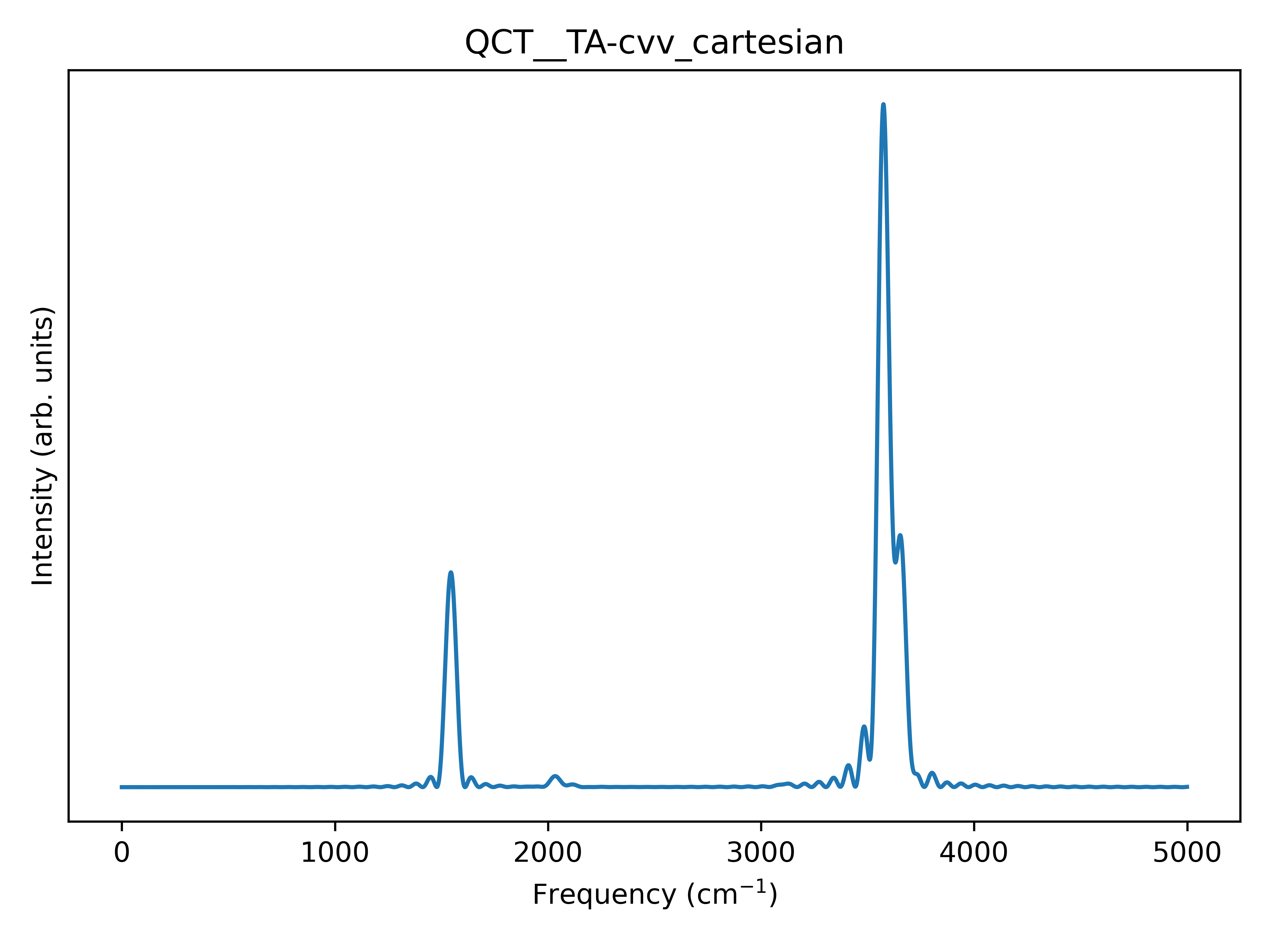
Classical spectra
Finally, it’s time for Flying Nimbus. We want the full cartesian spectrum, so we run:
python flying_nimbus.py --coord cart --plot --plot-dpi 600 \
 --xyz h2o_opt.xyz --hess Hessian_flat.out \
 --traj parsed_log_traj.xyz --norm1
this should give us the following .png image: