Gaussian tutorial
A simple, beginner-friendly guide to the Flying Nimbus programs.
The big picture
These tools work together as a pipeline:
Bulma → Vegeta → Flying Nimbus
Bulma prepares files from quantum-chemistry data.
Vegeta uses the optimized structure and Hessian to build velocity and mode-related outputs.
Flying Nimbus reads trajectory-based data and turns it into spectra that you can compare, export, and analyze.
Quick overview
Program |
Main job |
Typical inputs |
Typical outputs |
|---|---|---|---|
Bulma |
Build inputs and extract useful files |
XYZ geometry, Gaussian/ORCA/Q-Chem outputs |
optimized XYZ, Hessian files, BOMD/OPT/FREQ input |
Vegeta |
Build velocity and mode-related outputs |
equilibrium XYZ, flat Hessian |
|
Flying Nimbus |
Compute, compare, and analyze spectra |
equilibrium XYZ, trajectory, Hessian, |
plotted spectra, CSV export, peak metrics |
Bulma GUI Tutorial
Bulma is the preparation tool. This is where you usually:
create an optimization or frequency input
extract the final optimized geometry
extract the Hessian
prepare BOMD inputs
and, if needed, convert BOMD data into files that are easier to use later in Flying Nimbus
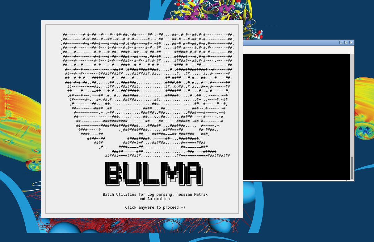
Bulma splash screen.
How about the GUI
The most important ideas are simple:
Choose the working directory first
Use the left sidebar to switch between Opt, Hessian, BOMD, and About
Use the Help panel on the right whenever a field name is unclear
Always check the Log panel at the bottom after you run something
If you are unsure about a field, keep the default and only change the options you understand.
Step 1 — Create an optimization or frequency input
On the Opt page, start by selecting the workdir. Then choose the software row that matches your code, such as Gaussian, ORCA, or Q-Chem.
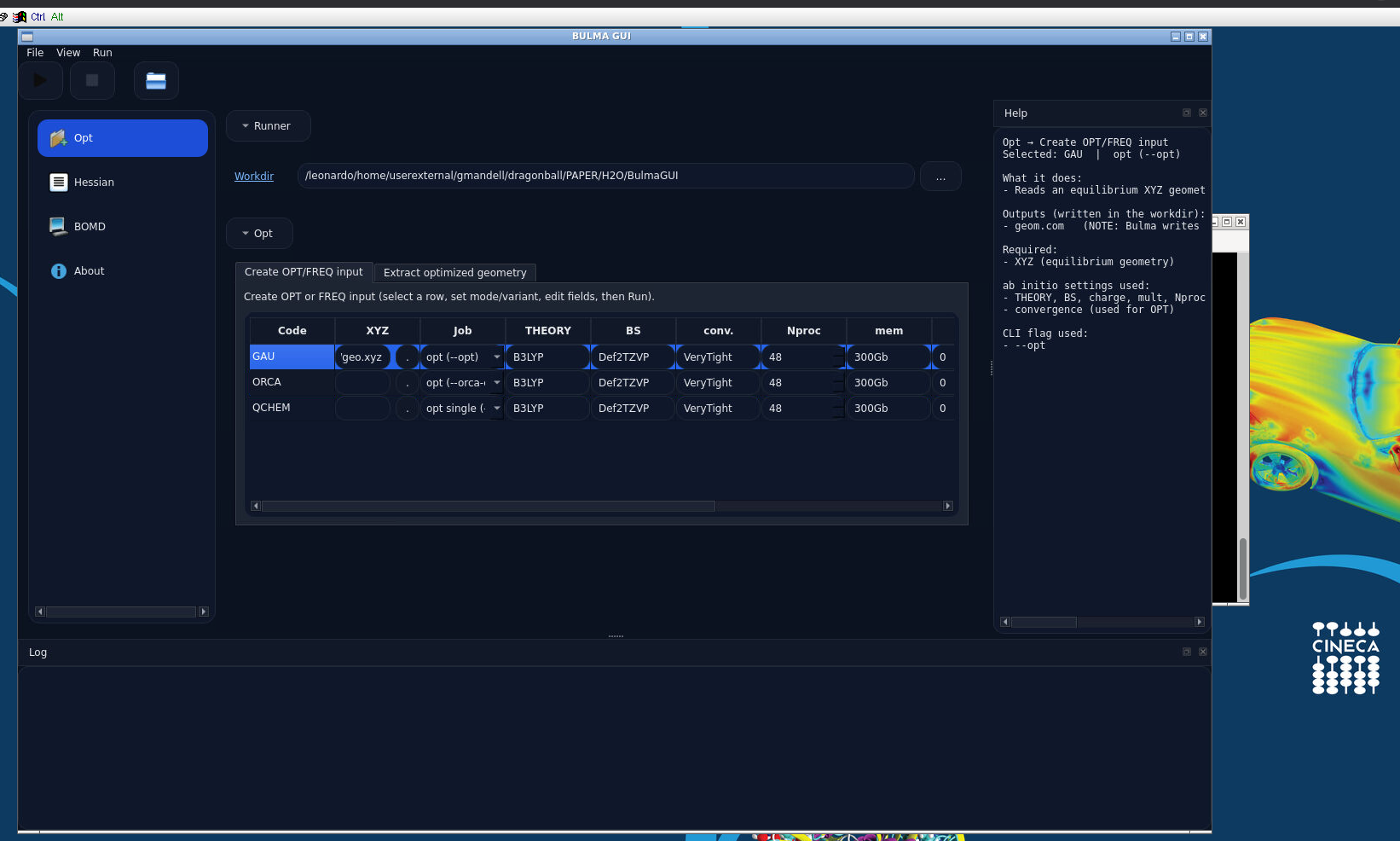
Bulma Opt page. The working directory is at the top, the software-specific settings are in the middle, the help panel is on the right, and the log is at the bottom.
As a beginner, focus on these fields first:
geometry input file
job type
theory
basis set
charge
multiplicity
number of processors
memory
optional dispersion
A completed example looks like this:
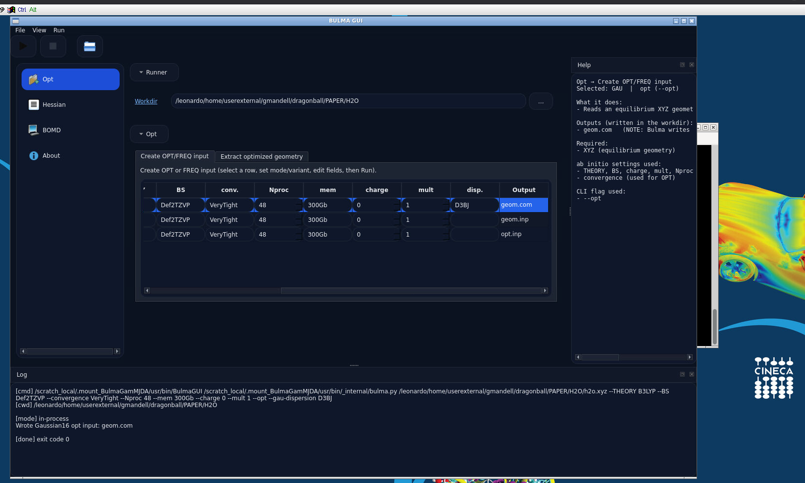
Completed Bulma example. The log confirms the command and the file that was written.
What to check after clicking Run
The log should finish cleanly
The output file name should appear in the log
If nothing is written, the first things to check are the workdir and the input path
Step 2 — Extract the optimized geometry
Inside Opt, Bulma also lets you extract the last optimized geometry from a finished output file. This is useful when you want a clean .xyz file to pass to Vegeta or Flying Nimbus.
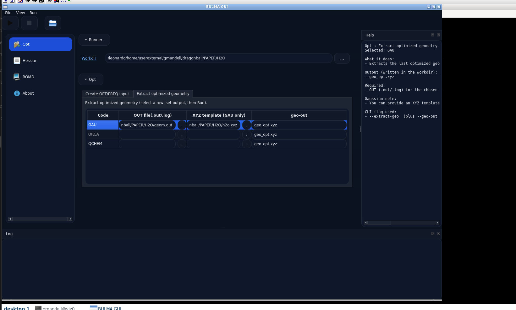
Bulma can extract the optimized geometry into a new XYZ file.
Step 3 — Extract the Hessian
Use the Hessian page when you need the Hessian matrix and its flat-vector version. The flat version is the one Vegeta typically uses later.
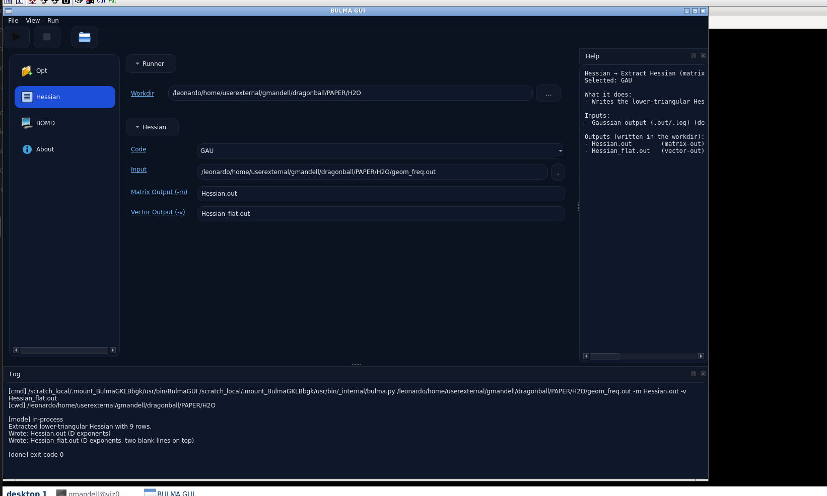
Bulma Hessian extraction page.
A good beginner rule is:
keep both outputs if possible
label them clearly
and store them in the same working directory as the optimized geometry
Step 4 — Generate a BOMD input
The BOMD → Generate tab is where you build a dynamics input from an equilibrium geometry and a velocity file.
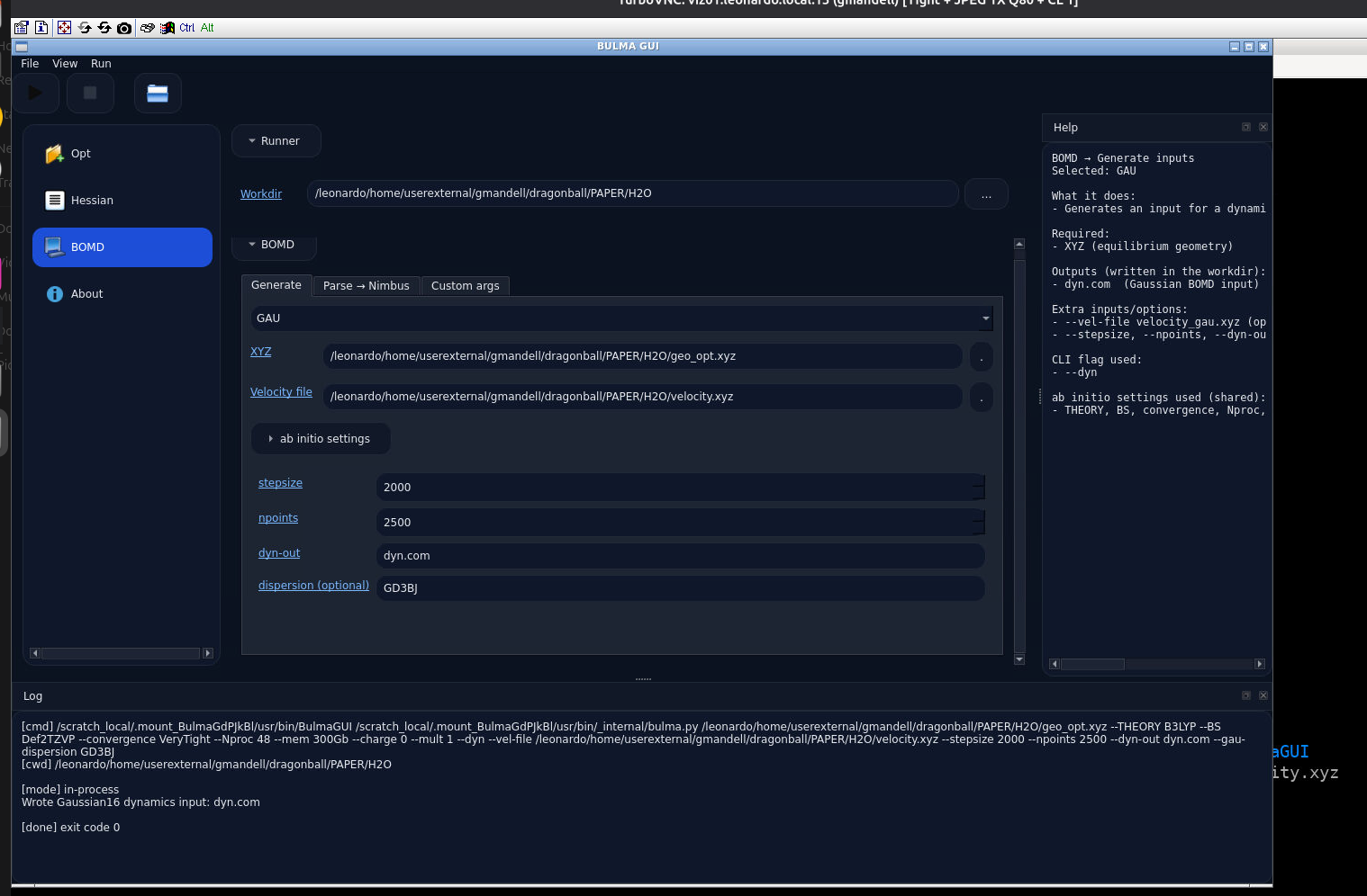
Bulma BOMD generate page.
The fields you will usually care about most are:
XYZ: the equilibrium geometry
Velocity file: usually the file produced by Vegeta,
stepsize
npoints
dyn-out
optional dispersion
and the shared ab initio settings
A safe beginner order is:
prepare the geometry
prepare the velocity file
then generate the BOMD input
Step 5 — BOMD → Parse → Nimbus
The Parse → Nimbus tab converts BOMD-style outputs into files that are easier to use in Flying Nimbus.
This tab is especially useful when you already have a finished dynamics run and want to move from raw trajectory-style output to spectral analysis.
Pay attention to:
the selected parser type
the input log or output file
the equilibrium geometry template if requested
the frame range
the base name for the generated outputs
and any optional energy export
A good beginner habit is to keep the output base name simple and descriptive, because you will see that name again later in Flying Nimbus.
Step 6 — BOMD → Custom args
The Custom args tab is the advanced escape hatch.
Use it when:
the GUI does not expose the exact option you need
you already know the command-line syntax
or you want to reproduce a command exactly
As a beginner, only use this page when the normal tabs are not enough. If you do use it, copy the command carefully and test with short runs first.
Common beginner mistakes in Bulma
Forgetting to set the workdir
Using the wrong output file when extracting the optimized geometry
Sending the wrong Hessian file to Vegeta
Mixing files from different molecules or different calculations in the same folder
Changing too many advanced settings at once
Vegeta GUI Tutorial
Vegeta sits between Bulma and Flying Nimbus. It uses the optimized structure and Hessian to generate velocities and other mode-related outputs.

Vegeta splash screen.
Step 1 — Files page
The Files page is where you load the key inputs.
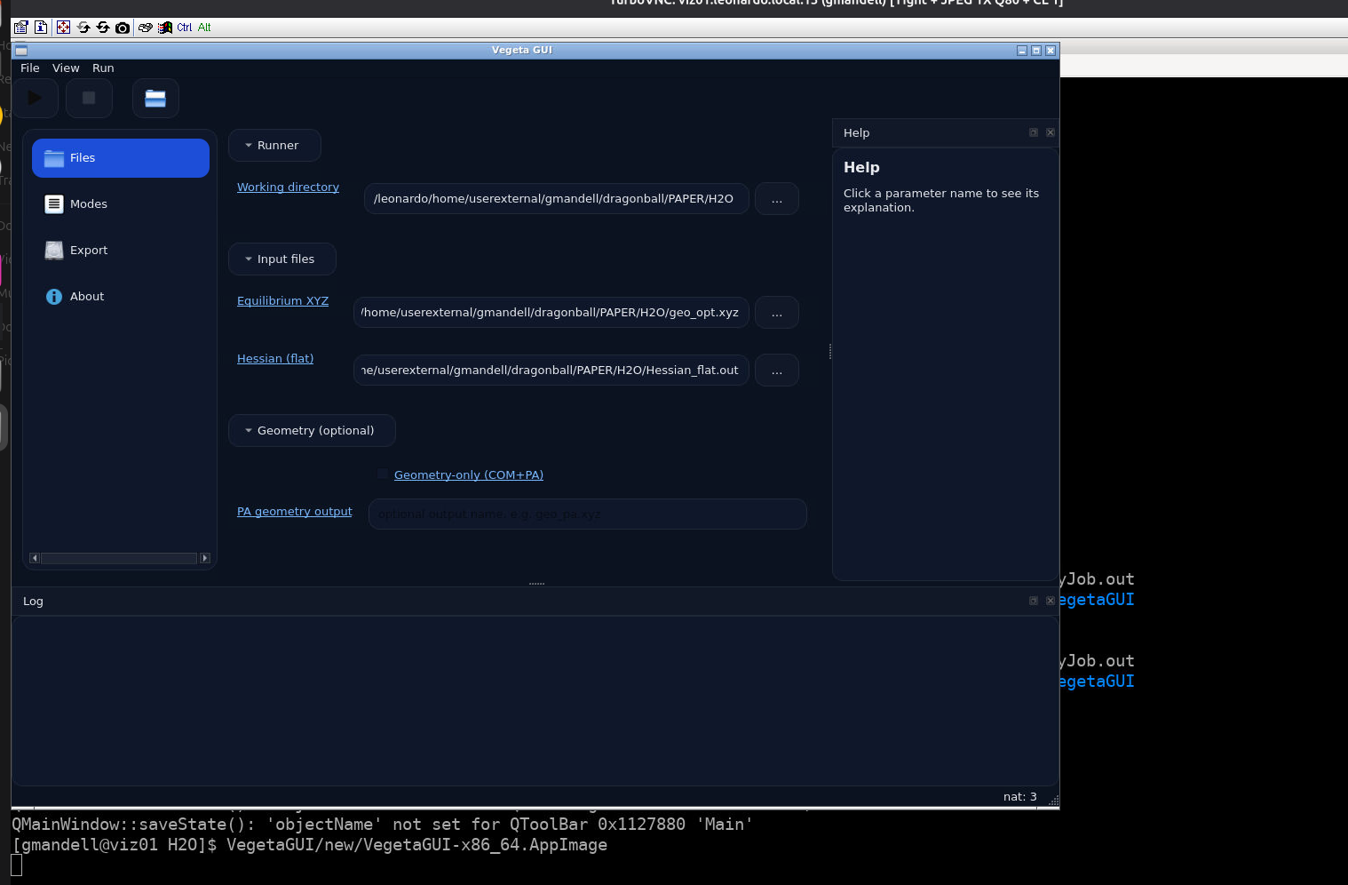
Vegeta Files page.
The most important fields are:
working directory
equilibrium XYZ
flat Hessian
optional geometry-only output
For a first run, keep it simple: load the optimized geometry from Bulma, load the flat Hessian from Bulma, and leave the optional output fields alone unless you know you need them.
Step 2 — Modes page
The Modes page is where the main configuration happens.
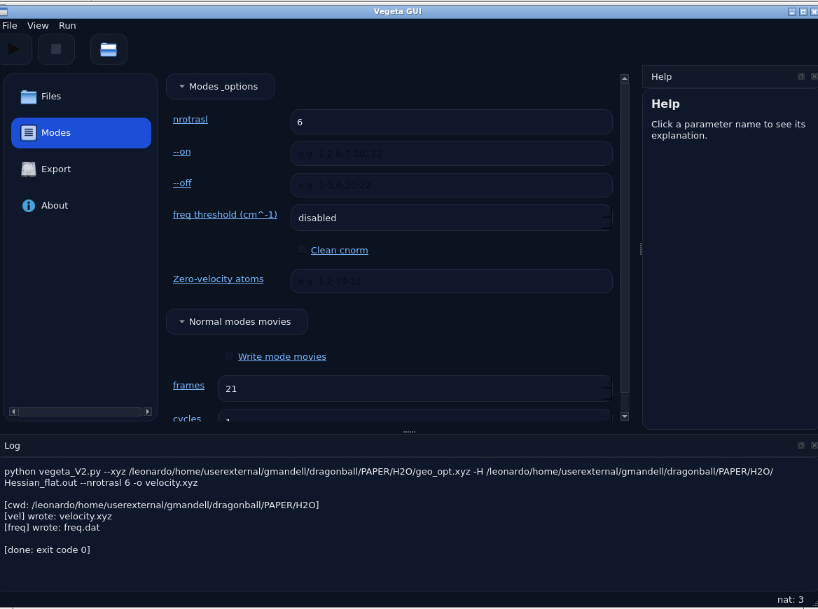
Vegeta Modes page.
Here is how to read it:
nrotrasl controls how translational and rotational modes are handled
on and off let you excite specific modes or switch them off
freq threshold can be left alone at first, it is used to remove low frequency modes below the threshold
zero-velocity atoms is useful only when you deliberately want some atoms to have zero velocity
normal modes movies is optional and mainly for inspection and visualization
Step 3 — Export page
The Export page controls the output names.
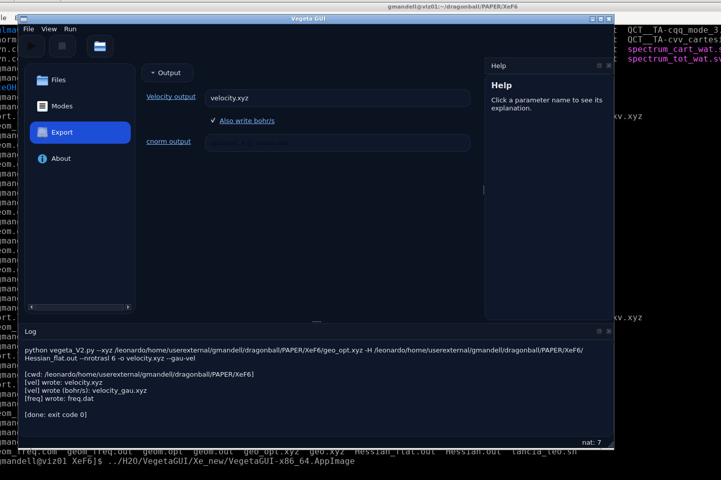
Vegeta Export page after a successful run.
The main outputs are usually:
velocity.xyzoptional bohr/s velocity output
optional
cnormfilefrequency information written to the working directory
What you usually keep from Vegeta
a velocity file for later dynamics work
frequency information (freq.dat)
an optional
cnormfile when Flying Nimbus needs it
Common mistakes in Vegeta
Using the wrong geometry for the Hessian
Mixing Hessians and structures from different jobs
Excluding or exciting modes without keeping track of what was removed or excited
Flying Nimbus GUI Tutorial

Flying Nimbus splash screen.
Flying Nimbus is the analysis and visualization tool. It reads structural and dynamics information and turns it into spectra that you can compare and analyze inside the GUI.
Presets
At the top of the GUI, Flying Nimbus includes Load preset and Save preset buttons.
These are useful when:
you repeat the same analysis often
you want to save a known-good setup
or you want to compare different analyses without retyping everything
Step 1 — Files page
The Files page collects the core inputs.
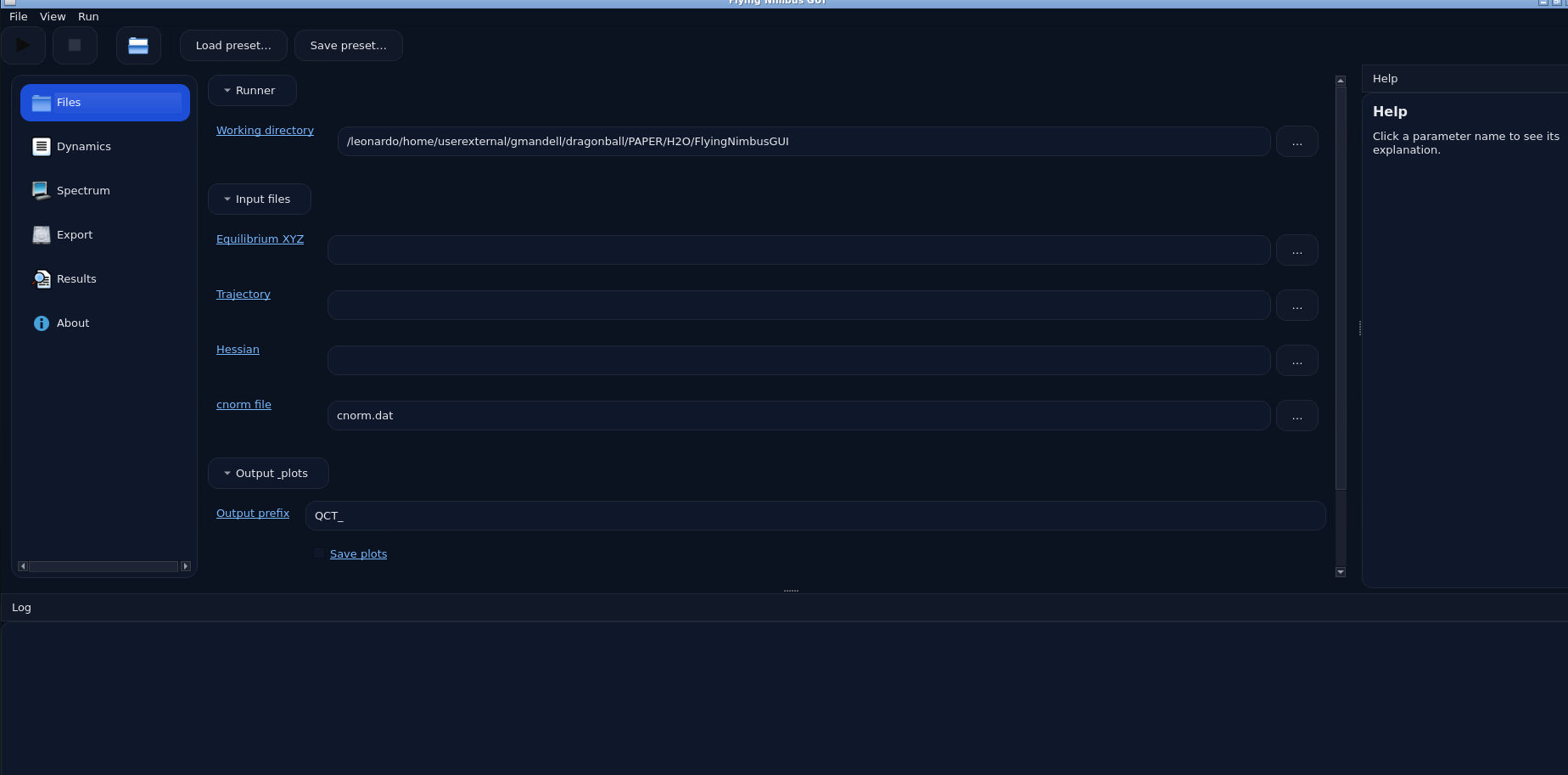
Flying Nimbus Files page.
The key inputs are:
working directory
equilibrium XYZ
trajectory
Hessian
optional cnorm file
output prefix for plots
Step 2 — Dynamics page
The Dynamics page controls how the trajectory file is interpreted.
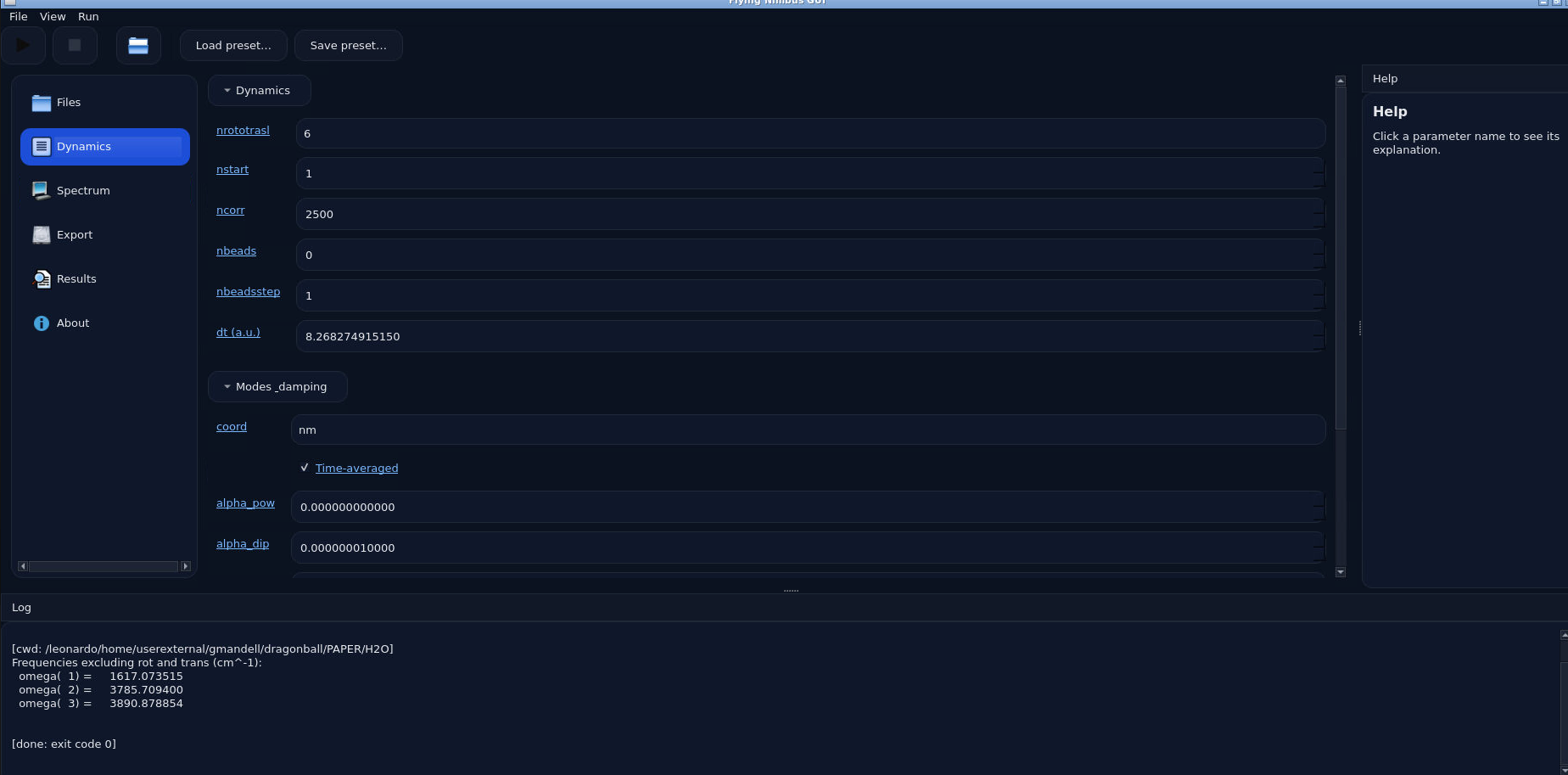
Flying Nimbus Dynamics page: upper part.
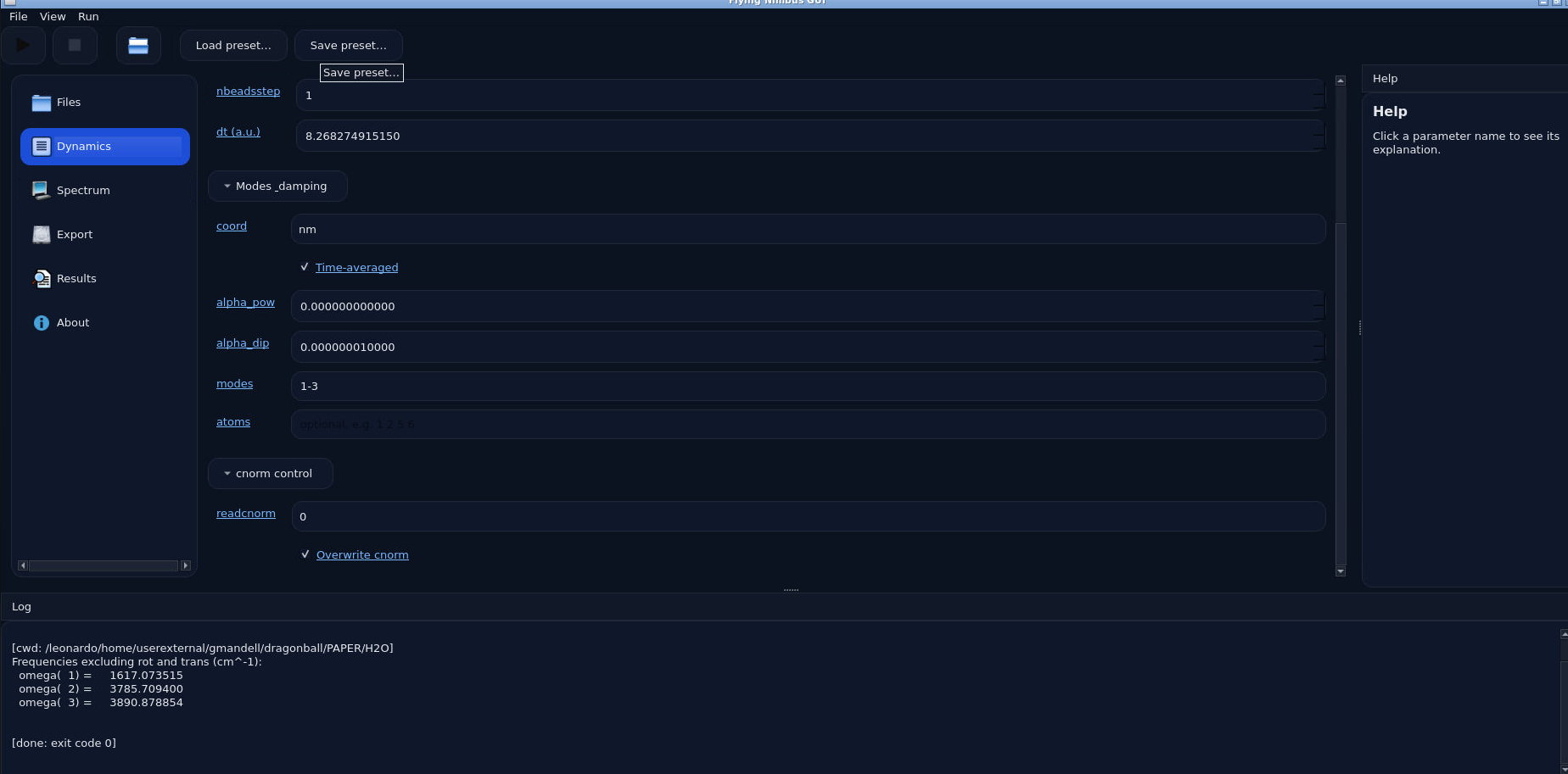
Flying Nimbus Dynamics page: lower part.
Treat this page in two layers:
The basic layer
Start with the main run settings shown in the screenshots, such as:
nrotraslnstartncorrnbeadsnbeadstepdt
For Gaussian trajectory files and non-linear molecules, the default values are usually fine.
The selective-analysis layer
The lower part lets you narrow the analysis.
Common examples:
select only specific modes
select only specific atoms (atomwise spectra)
choose whether the calculation is done in normal-mode or Cartesian form
choose whether you want time averaged spectra or not (TA). We recommend using TA as default
reuse or overwrite the
cnormfile
Step 3 — Spectrum page
The Spectrum page controls the spectral grid and simple post-processing.
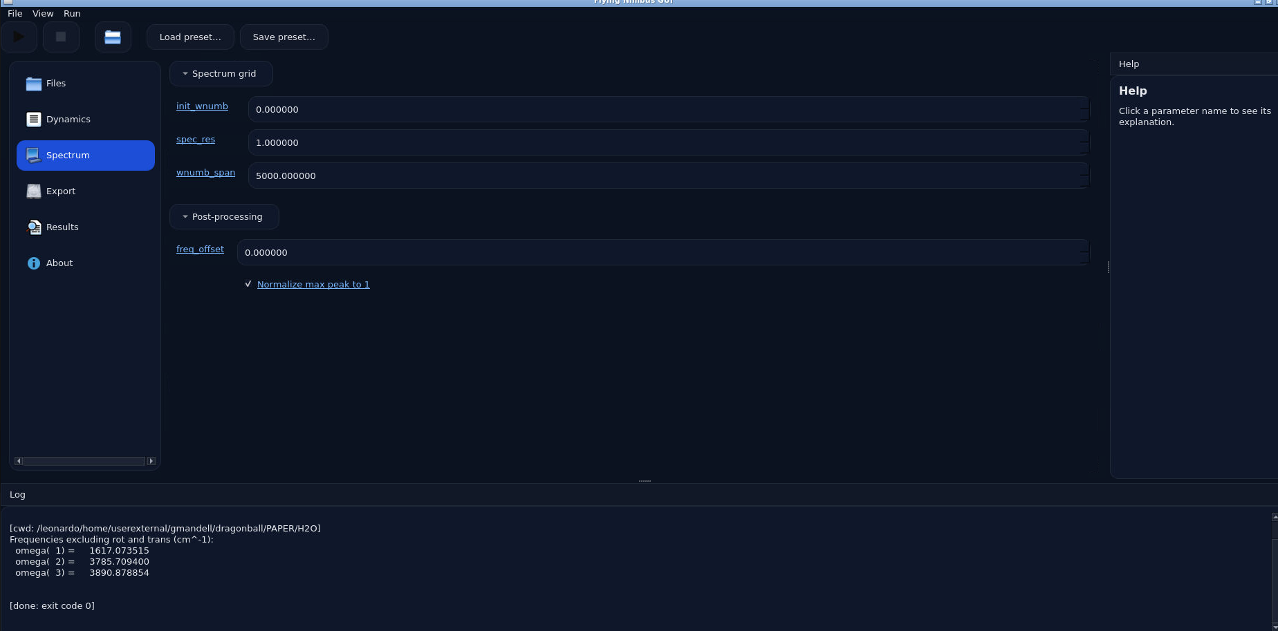
Flying Nimbus Spectrum page.
The most important fields are usually:
initial wavenumber
spectral resolution
total wavenumber span
frequency offset
normalization of the highest peak
For a first pass, keep the setup simple and only change the range or resolution when you have a clear reason.
Step 4 — Export page
The Export page controls CSV and other export options.
writing CSV output
choosing the delimiter
exporting merged CSV data when you want a single combined table
This page is especially useful when you want to move the processed spectra into Excel, Origin, Python, or another plotting tool.
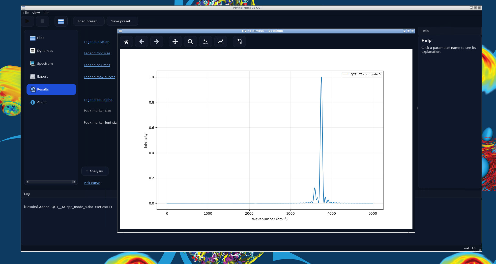
Step 5 — Results page
The Results page is where comparison and interpretation happen.
Loading spectra and organizing series
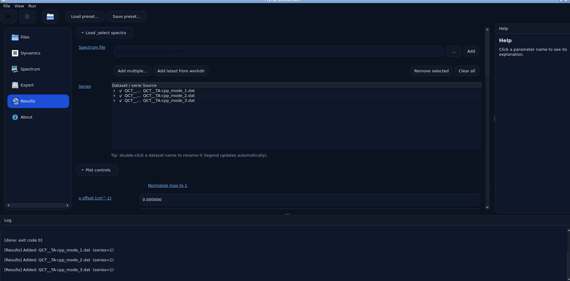
Flying Nimbus Results page: loading spectra and organizing series.
This is where you:
load one or many spectra
group them into series
rename datasets
decide which curves should appear together
Plot controls
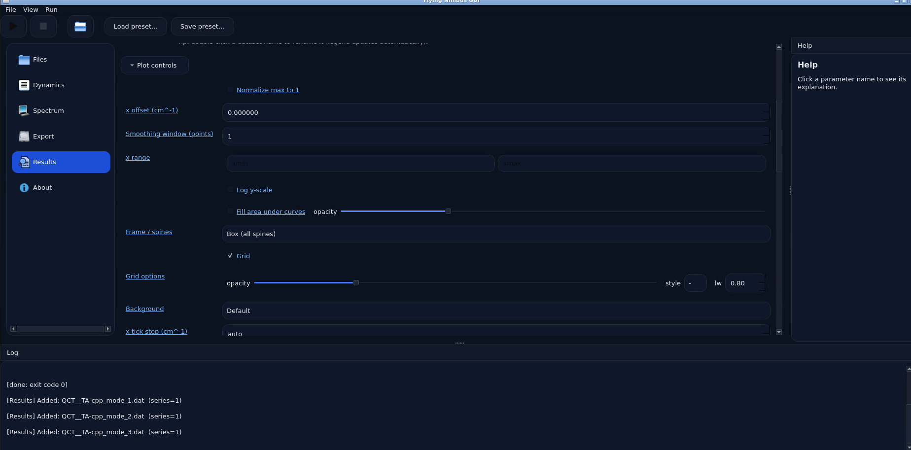
Flying Nimbus Results page: plot controls.
Useful controls include:
normalization
x offset
smoothing window
x range
log y scale
filling the area under curves
grid options
frame or spine settings
background
legend settings
These controls are extremely helpful for making comparisons readable.
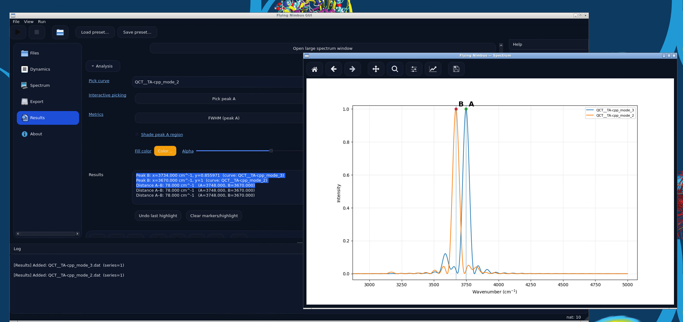
Analysis controls
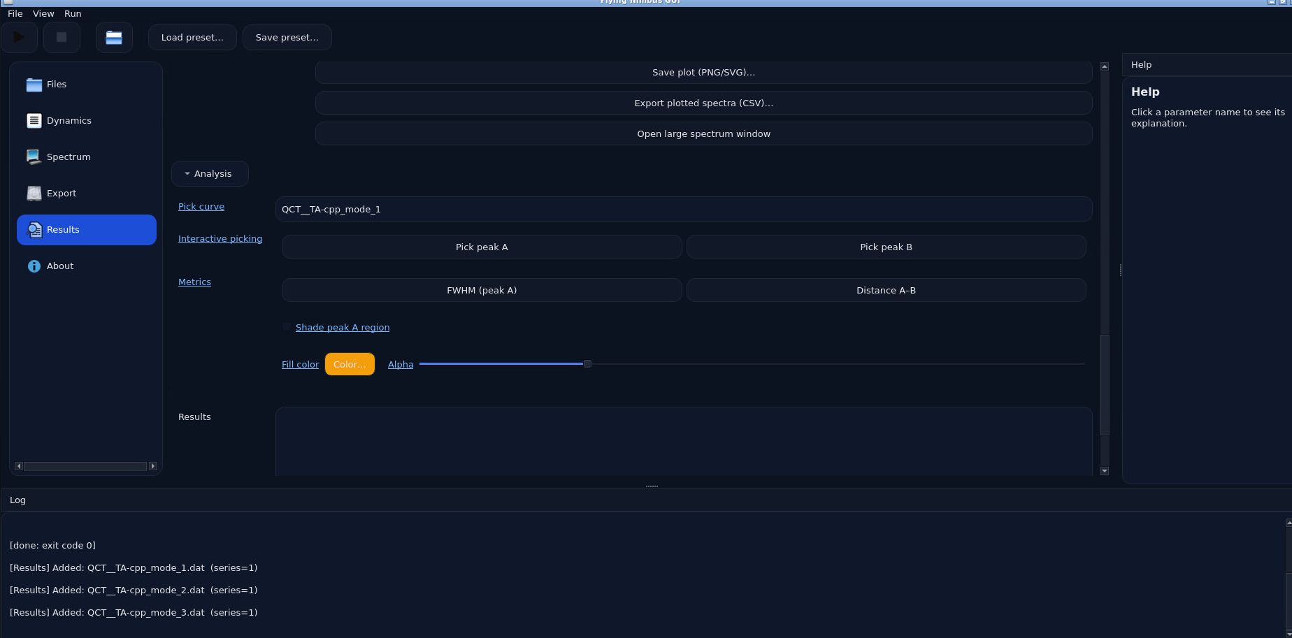
Flying Nimbus Results page: analysis controls.
This part of the page lets you:
select the active curve
pick peak A
pick peak B
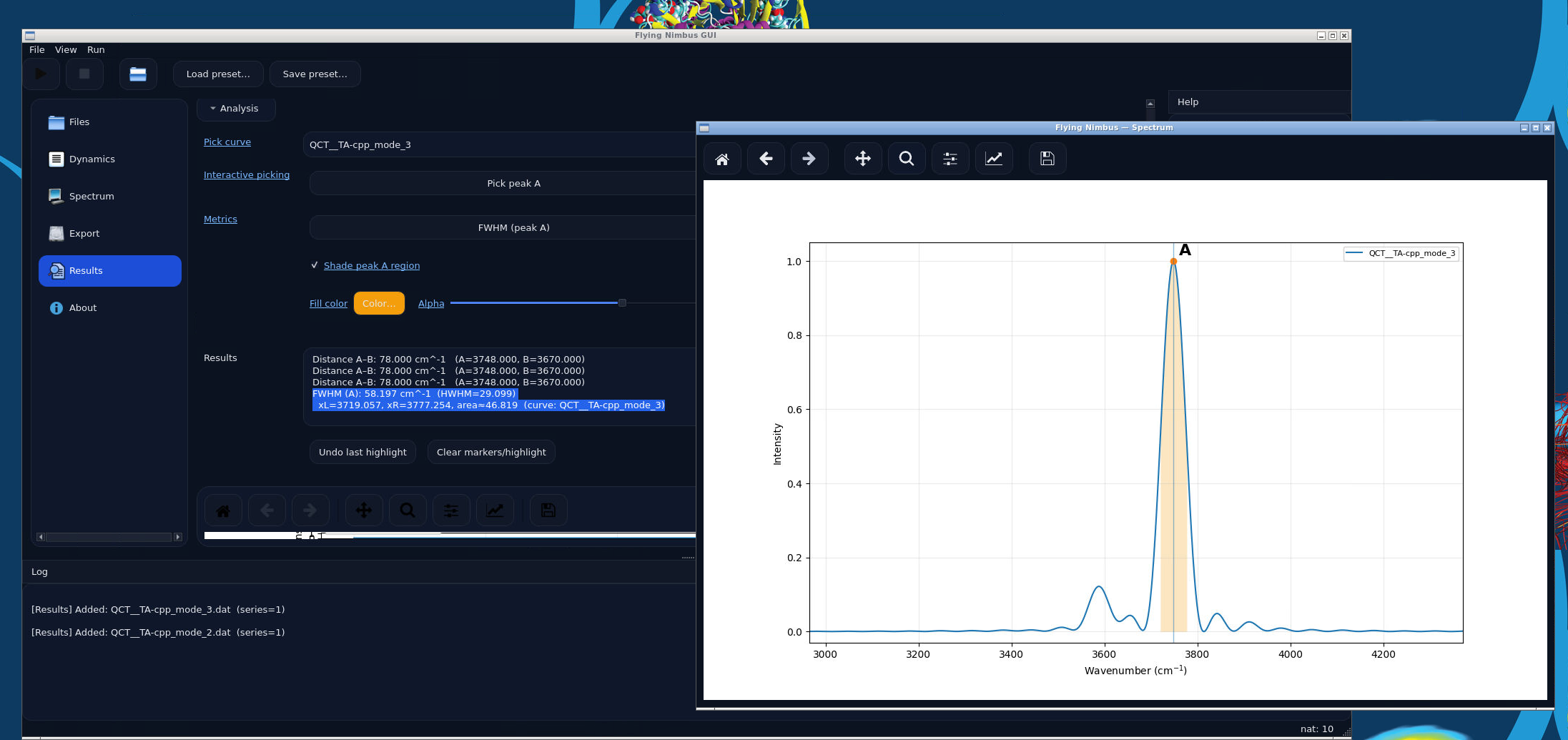
compute FWHM for peak A
measure the distance A–B
shade the region around a selected peak
save the plot
export the plotted spectra
Example: shaded peak region, FWHM resuls, peak-peak distance
Common mistakes in Flying Nimbus
Loading a trajectory that does not match the equilibrium geometry
Reusing a stale
cnormfile without noticingComparing spectra with different scaling and forgetting to normalize
Measuring peak distances without checking which curve is currently active
Exporting a plot before checking the x range and legend