ORCA Tutorial

Optimization and Frequency

Let’s take a guess geometry for the water molecule and put it in h2o.xyz:

3

H   0.76144678642012      0.42041157793785     -0.21139612912752
O   0.00092389677508     -0.10975434825824      0.05112764711589
H   -0.76825069319520      0.42203277032039     -0.18105150798837

For the sake of this tutorial, we will divide the optimization and frequency runs, even if ORCA allows to run both optimization and frequency jobs from a single input. We create the opt input with bulma:

python bulma.py h2o.xyz --orca-opt

This will generate the file orca_opt.inp. We run the optimization. When it is done, we extract the final geometry with (the .out file should be in your output folder)

python bulma.py orca_opt.out --extract-geo --geo-out h2o_opt.xyz

We now generate the (optimization) and frequency input by running

python bulma.py geo.xyz --orca-freq

and we run the frequency job. When the frequency job is terminated, we extract the hessian file (the .hess file should be in your output folder):

python bulma.py geom_freq.hess --orca-hess

We can now move to the harmonic analysis with vegeta.

Initial Velocities

This step is common for all the ab initio codes. We run vegeta.py with the optimized geometry and extracted Hessian matrix:

python vegeta.py --xyz geom.xyz -H Hessian_flat.out -o velocity_orca.xyz

We can check that everything went smoothly by comparing the freq.dat output file with the one provided in the repository. NB: For ORCA, bulma expects the initial velocities in a file called velocity_orca.xyz, since velocity.xyz is the default output for ORCA trajectory velocities.

Classical dynamics

We now can generate the input file for the classical dynamics run. Using bulma:

python bulma.py h2o_opt.xyz --orca-qmd

This will generate the files h2o_opt_qmd.inp and h2o_opt_qmd.mdrestart. We can run it. When the dynamics is done, we extract the trajectory file using bulma:

python bulma.py dummy_input --parse-orca-qmd

For ORCA, bulma reads the trajectory.xyz and velocity.xyz files, so the dummy_input string is required to satisfy the positional input of the CLI. The trajectory is written in the file parsed_log_traj.xyz.

Classical spectra

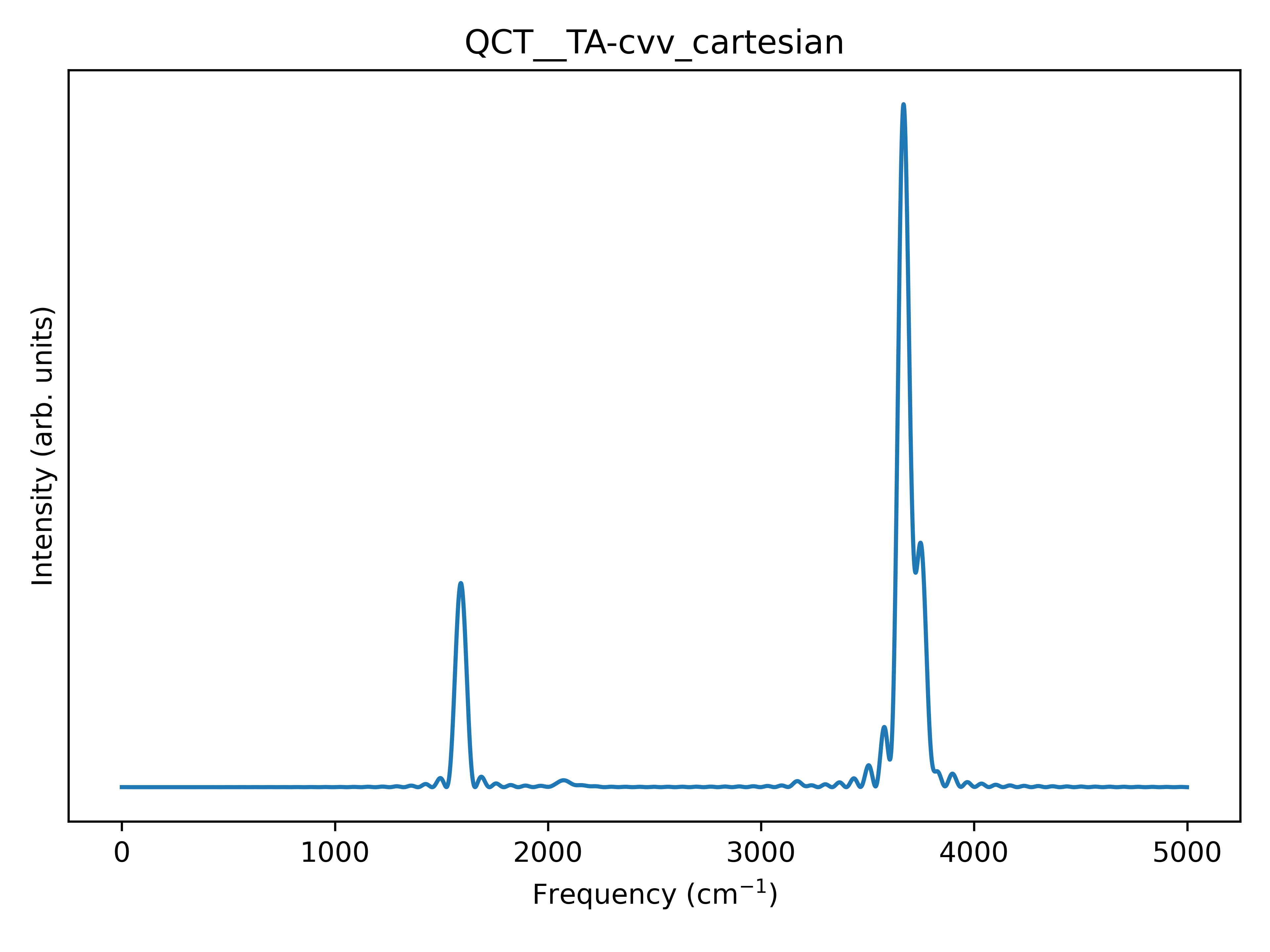
Finally, it’s time for Flying Nimbus. We want the full cartesian spectrum, so we run:

python flying_nimbus.py --coord cart --plot --plot-dpi 600 \
 --xyz h2o_opt.xyz --hess Hessian_flat.out \
 --traj parsed_log_traj.xyz --norm1 

this should give us the following .png image: